IPC

I recently found an interesting discovery.  The new platform of SAP S/4 will no longer support the IPC.  I this very interesting as SAP has spent so much time and effort to build this better platform, but currently according to OSS, there is no plan to integrate it.  If any of you out there have heard the plan in the CWG, please let me know.

The concept is that since IPC is java based, and HANA/S/4 have no concept of Java…  so it means that within S/4 you cannot select a configurable material and make it IPC to look nicer.

Would love to hear any input on this, I was certainly disappointed.

Thanks for reading,

Well, a while back, I did some posts about different ways to debug in the IPC.  THere was one more way that I never talked about, mostly because I hadn’t been able to get it working on my machine.  Using the SCE Debug as a tool is a great way to test your models on a local machine.  While it won’t contain all the same information as doing it online, it does give you the opportunity to play with your model without being connected to SAP or even the internet.

The modeling happens in R/3 as usual. If something is to be tested in IPC, a runtime version has to be created. This is of course the same pre-requisite for the IPC running in VMC of ECC. However instead of calling the report to publish the runtime version to VMC’s DB, you download it, using transaction CU36. It will download the whole KB into flat files. The flatfiles will then be imported into a (local) database. This process is executed by a simple batch file. After the flatfiles are imported, the RTV is available to SCE.  For more information on this, see my previous posts.

Select from the menu Trace–>Trace Settings.

In the dialog you can select an appropriate input level for filtering out some details (if wanted). 9 will show everything, which makes sense for a trace.

Select from the list of modules, for what you want to receive log entries. They are as follows:

Module	Description
DDB	Dynamic Database. This is the memory of the inferencing engine, storing all facts about the current configuration state.
PMS	Pattern Matching System. Constraints are considered declarative. This means in opposite to procedural coding where everything is executed line by line, constraints describe a status and will be executed in any undefined order if their pattern is fulfilled. The pattern usually exists of an object declaration as well as a condition. The pattern matching system is responsible to find those constraints, which patterns are fulfilled.
CSTR	Constraint. This is useful for figuring out for example in combination with DDB, how a constraint influences facts.
RULE	Rules. (If used) Mainly used in Advanced mode as monitoring rules
CFG	Configuration
SCND	Selection condition (good for troubleshooting existence or missing items on a bom explosion). See super bom.
PCND	Precondition. If used. It is strongly recommended not to use any preconditions.
PROC	Procedures. This option makes most sense in combination with DDB, seeing which modifications happen.
FUNC	Functions
TABL	Variant Table access

Table 1 “traceable engine modules”

Very typical and useful settings are DDB,CSTR,PROC. Eventually SCND if the bom explosion is to be verified.

After selecting the options, you can do any modification directly in the SCE UI. With each selection / modification, you see traces being updated in the lower part of the window:

The trace area is not very powerful regarding functionality like search etc. The right click menu allows to clear or to save it to a file. It is however possible to select all entries with ctrl + A, copy the traces (ctrl + C) and paste them into an external editor, such as notepad++.

One of the biggest benefits of using the SCE over using IPC is if you want to see the initial logic being executed, you activate the trace and create a new configuration session (with the white paper icon in sce).  The IPC will automatically execute the initial logging before you can begin the simple trace, so often this will help you find problems within the initial execution of your dependencies.

As always, Thanks for reading,

Well, since I’m on a roll, figured I might as well show you how to load the KB into the SCE UI within your local database.

The first step is to make sure that you extracted the latest files from CU36 (see my previous post for details on this).

Now, here is where you need to do a little work.  In your IPC installation directory (and I use the word installation loosely, since it was just a zip file with a bunch of files).  So, what needs to happen is to copy all the flat files into the ..\db directory (for me, there was an intermediate folder, so for me it ..\db\temp\ to hold all my flat files.

Now, one additional step that I needed to do was copy the file sce_import_meta_data.sql from the ..\lib\scripts\ directory and place it in the ..\db\ directory (notice that even for me, it was not in the temp directory).  Now, I also needed to rename this file to be: import_meta_data.sql

Once this prep work has been completed, go the ..\bin\KBAdmin.bat

Verify your DB settings (see my previous post on the SCE if you need more details on how to set this).

Use the menu:  knowledgebase–>upload

enter in the location you used for the flatfiles (see above for more details).

Press Start Upload.

When it’s done, you will now have the DB populated with the knowledge base you loaded.

When you know what to do, it’s pretty easy…  but this took me a few hours of experimenting to figure out what to do… =)

Thanks for reading,

Well, now that you know how to get the database setup for the SCE UI, you need to work on creating the knowledgebase.  This is pretty straightforward exercise, but it does require a few transactions to perform the whole process.  Let’s walk through what you need to do.

We start with Transaction: CU31 to create the KB object.

Much of the information is just descriptive, so set the status and give it a description.  THen press the profiles button.

Again, these are just names, so name the Profile and give it a description.  Then press enter.

Now, we finally get to some real data.  I typically enter in the KMAT material, but you could do it by class and class type.  Add a description and then save.

Now that you have a knowledge base, you can create the runtime version (RTV).  Go to transaction CU34.

IN this screen, we set up all the vital stuff, including what plant the BOM should be looking at, if it’s a production BOM or Sales BOM, etc… Also, a very important field is the valid from date.  Remember, that KB’s and RTV’s have no concept of engineering change.  This means that the valid from date is VERY important for your process going forward.

After you enter in the info, I encourage you to check.  Press the syntax check button, and you will receive a report of your model.

My model is very simple, so everything is green.  If anything is yellow, be sure to pay close attention.  This could cause you issues within the SCE/IPC.  The question mark to the right often has good information.

Finally, green arrow back, press generate, and you have your RTV.

The last step is just to download the flat files.

Use transaction CU36

Enter in your KB and version, then press the export button.

The only field you need to be concerned with here is the Path.  the rest only applies if you are using R/3 or CRM as the your SCE installation.  For my purposes, I’m focusing on the offline database only.

Hit the green check and you’re ready,  Next post I’ll talk about uploading the flat files into the SCE.

Thanks for reading,

Now, I struggled with this one for a while.  I was able to get the IPC 4.0 files that include the stand alone version of the SCE UI.  I recently learned that in all the versions after 4.0, this option is no longer available.  So, to me, 4.0 is still a premium, just to be able to do the offline testing of a model (especially for someone that periodically travels on airplane.  ha ha ha).  Anyway, after some digging, I was finally able to figure out how to get this installed.  If you’ve read my previous posts on the SSC installation, you’ll remember that you need SQL Server on your local machine in order to make this work.   Please refer back to this post if you are having issues connecting.

Now, the first thing you need before you can do anything is set the system variable for JAVA_HOME.  If you aren’t familiar with this, following the next couple of steps.
Right click on my computer, and select properties.  If you are in windows 7, click the advanced system settings, and press the environment variable button.

The variable name needs to be: JAVA_HOME

the value is the path on your hard drive to get there.

Now, once you have this, you can move on to the harder pieces.

The next thing you need to do is locate the files for the ipc, and go to the /bin directory.  This will have a bunch of batch files.  The first file you need to execute is:  admin.bat

The first screen, you can leave this defaulted as it is.  This would be more important if you wanted to connect directly to R/3 or CRM.  Go ahead and press Next. and then Next again, since you don’t need to worry about security on your local machine 🙂

this screen is where all the work comes in.  Press add to add a new connection

Now, all of these values will come from the SQL Database you created.  See SSC installation for more details.  Be sure to create a new database, I called mine IPC.  Then populate all the other values.  The Port you can accept the default, for Client, you can just use 000 since it’s local.

Finally, make sure to highlight the new DB you added, and press the Create Tables button.  Then press save.

I’ll take more about this soon, including how to upload a model into the stand alone database.

Thanks for reading,

This next method is yet another option for IPC Tracing.  This time we talk about the Engine Tracing.  First things first, you have to turn it on.

Activating engine traces

In transaction SM53, select Log Configuration:

Activate log level “Debug” for:

• com.sap.spc.document.rfc.engineTrace
• com.sap.sxe.trc.imp

From now on, engine traces will be logged and you can use IPC also from VA01.

For seeing these traces, go back to SM53, Display Log and navigate to com.sap.sxe.trc.imp.

This will bring up the engine traces.

Now in comparison, this eliminates the issue of seeing the configuration initialize.  However, it comes with a price.  You MUST Always turn back the log level to error after you are done. VMC logging is very rudimentary and traces produce a lot of data. Complete instances can be brought down by consuming all harddisk space  with log files!  So unless you want to crash your IPC, do NOT leave this on.

thanks for reading,

 

As I mentioned in a previous post, there are 3 main ways to debug or trace in the IPC.  This second method is probably the easiest method, but comes with limitations (doesn’t everything 🙂 ).  IPC Tracing using IPC UI is very useful and very simple to see what’s happening within your configuration.

Step one is to activate the tracing functionality.

The IPC UI has a built in functionality to display engine traces. In order to active these engine traces, you have to turn on the following switch in the XCM Administrator:

Select or create a specific component configuration for Behavior.

The option behavior.enabletrace is by default off (“F”) and has to be turned on (“T”).

Once traces have been activated, there is a new option in the menu “Trace UI”.

The trace settings can be specified on the following screen:

The modules are the same as in SCE, see Table 1 “traceable engine modules” .

Activate the traces by clicking “Apply Trace Settings” in the top menu.

This brings you back to the configuration UI, now click on Trace UI again and you will see a trace similar what was shown in the COM_CFG_SUPPORT.

Now, I mentioned a downside to this approach.  That downside is that it’s impossible to ever see the initialization of your characteristics and values.  You can see what happens when things change, but not the values that get set upon entering the configuration, like reference cstics.  For any development environment, I still highly encourage this setting to be turned on.

thanks for reading,

My next couple of post will talk about how you can use the IPC Trace functionality.  There are several different ways you that you can trace the dependencies and constraints within the IPC, and today I’ll talk about the first one, COM_CFG_SUPPORT.

Tracing with the transaction COM_CFG_SUPPORT is always available and requires the least effort in the sense of installing any kind of component. However it has the drawbacks of an ugly configuration ui and have to do all steps manually.

The first step to Tracing a configuration session is to figure out what the kbid for the knowledgebase is which you want to test. In order to do so, go to table: COMM_CFGKB in SE16/SE16N.  Pick the most recent KBID that fits your KB and RTV you are tracing.  Next go to COM_CFG_SUPPORT.

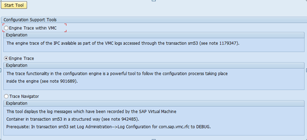
Select “Engine Trace” and click on “Start Tool”.

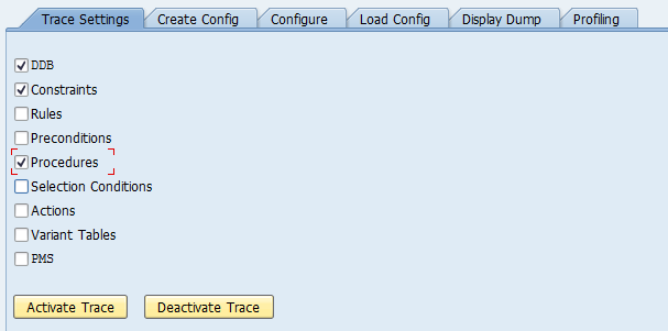
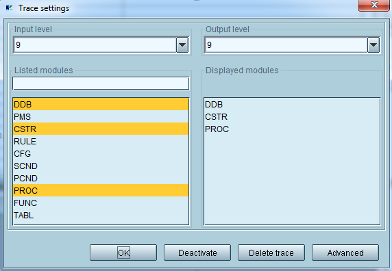
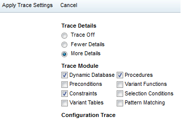
Select the engine module you are interested in and click on activate trace. For a brief list of what these engine modules mean, please have a look at Table 1 “traceable engine modules”.

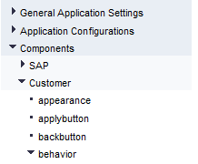
Then go to tab “Create Config”:

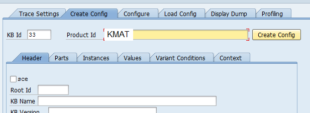
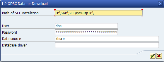
Enter the kbid (which we got from comm_scecfg) and the product id.

Click on Create Config.

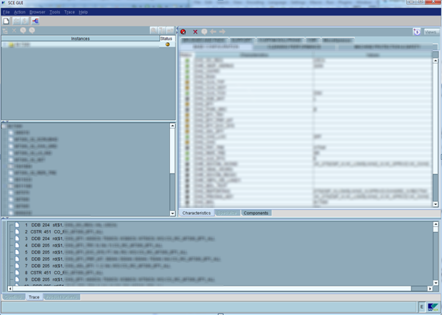
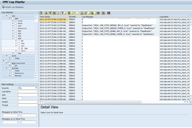
This will bring up the initial trace:

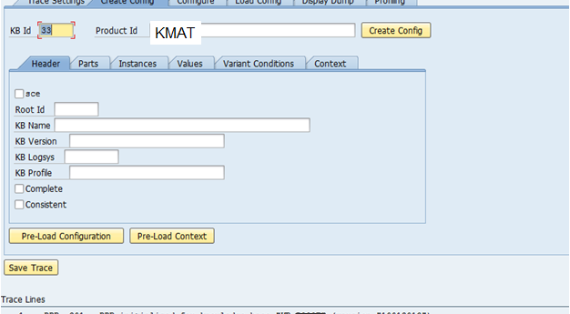
You’ll see some of the initial trace lines before anything happens.

1  DDB  201  DDB initialized for knowledge base “X” (version 0001)
2 DDB  219  Instance : “$1(product: XXX)” Created as Root
3  DDB 204 Fact : “sf($1, Cstic_1, INV_P, true)”: Inserted by “Classification”
4  DDB 204 Fact : “sf($1, Cstic_1, NOINP_P, true)”: Inserted by “Classification”

etc…  You’ll quickly start to recognize little things like INV_P is invisible, NOINP is no input, if it’s set by classification or  inferred by the system.

Now let’s set a characteristic value and this will actually show how painful the process is. Go to tab “Configure”.

We need to specify language independent names for the characteristic as well as for the value. The instance ID will be 1 (root instance).  Cstic name will be language independent name, and value is the language independent value.  Pretty straight forward.

Click on OK to set this value and see the trace underneath updating:

Now, you’ll see the new trace lines underneath, so you can see exactly what behavior occurs when you change or set a particular value.

Now, one of the big things to remember is that this won’t help you see what happens during the initialization phase in the sales order.  You’ll still have to simulate that yourself, which could be difficult.

Thanks for reading,